Statistical Analysis Using R

This post displays a use of the R programming language via the RStudio Integrated Development Environment (IDE) to compute test statistics and develop charts and graphs to draw conclusions about given data sets.

Code

#Alyssa Ball: Analyzing Data##############################################

#pacman installation + loading packages
if (!require("pacman")) install.packages("pacman")

Loading required package: pacman

Code

pacman::p_load(pacman,tidyverse,rio,reshape2,magrittr,BSDA)

#Import Data as Tibble Data Frame##########################################
dfo <- import("R5Data.xlsx") %>%
  as_tibble() %>%
  print()

# A tibble: 25 × 9
   Temperature Before After BrandOne BrandTwo Solution…¹ Solut…² Facil…³ Facil…⁴
         <dbl>  <dbl> <dbl>    <dbl>    <dbl>      <dbl>   <dbl>   <dbl>   <dbl>
 1        97.8    7.2   6.1      293      266        9.5    10.3      63      69
 2        97.2    7     6.5      286      243        9.4    10.6      57      65
 3        97.4    7.1   6.2      287      260        9.3    10.7      58      59
 4        97.6    7     6.1      271      265        9.6    10.4      62      62
 5        97.8    7.2   6.6      283      273       10.2    10.5      66      61
 6        97.9    7.3   6        271      281       10.2    10.3      58      57
 7        98      6.9   6        279      271       10.3    10.2      61      59
 8        98      6.4   5.5      275      270       10      10.7      60      60
 9        98.1    7.1   6.1      263      263       10.3    10.4      55      60
10        98      7.3   6.1      267      268       10.1    10.3      62      62
# … with 15 more rows, and abbreviated variable names ¹SolutionOne,
#   ²SolutionTwo, ³FacilityOne, ⁴FacilityTwo

Code

#Each Problem Assigned to an Individual Data Frame#####################################
df_prob1 <- dfo %>% 
  group_by(Temperature)%>%
  summarise()%>%
  print()

# A tibble: 16 × 1
   Temperature
         <dbl>
 1        97.2
 2        97.4
 3        97.6
 4        97.8
 5        97.9
 6        98  
 7        98.1
 8        98.2
 9        98.3
10        98.4
11        98.5
12        98.6
13        98.7
14        98.8
15        98.9
16        99

Code

df_prob2 <- dfo %>%
  group_by(Before,After)%>%
  summarise() %>%
  print()

`summarise()` has grouped output by 'Before'. You can override using the
`.groups` argument.

# A tibble: 13 × 2
# Groups:   Before [8]
   Before After
    <dbl> <dbl>
 1    6.4   5.5
 2    6.9   6  
 3    7     6.1
 4    7     6.5
 5    7.1   6.1
 6    7.1   6.2
 7    7.2   6.1
 8    7.2   6.6
 9    7.2   6.8
10    7.3   6  
11    7.3   6.1
12    7.7   7.5
13   NA    NA

Code

df_prob3 <- dfo %>%
  group_by(BrandOne,BrandTwo)%>%
  summarise() %>%
  print()

`summarise()` has grouped output by 'BrandOne'. You can override using the
`.groups` argument.

# A tibble: 11 × 2
# Groups:   BrandOne [10]
   BrandOne BrandTwo
      <dbl>    <dbl>
 1      263      263
 2      267      268
 3      271      265
 4      271      281
 5      275      270
 6      279      271
 7      283      273
 8      286      243
 9      287      260
10      293      266
11       NA       NA

Code

df_prob4 <- dfo %>%
  group_by(SolutionOne,SolutionTwo)%>%
  summarise() %>%
  print()

`summarise()` has grouped output by 'SolutionOne'. You can override using the
`.groups` argument.

# A tibble: 11 × 2
# Groups:   SolutionOne [9]
   SolutionOne SolutionTwo
         <dbl>       <dbl>
 1         9.3        10.7
 2         9.4        10.6
 3         9.5        10.3
 4         9.6        10.4
 5        10          10.7
 6        10.1        10.3
 7        10.2        10.3
 8        10.2        10.5
 9        10.3        10.2
10        10.3        10.4
11        NA          NA

Code

df_prob5 <- dfo %>%
  group_by(FacilityOne,FacilityTwo)%>%
  summarise() %>%
  print()

`summarise()` has grouped output by 'FacilityOne'. You can override using the
`.groups` argument.

# A tibble: 14 × 2
# Groups:   FacilityOne [10]
   FacilityOne FacilityTwo
         <dbl>       <dbl>
 1          55          60
 2          57          65
 3          58          57
 4          58          59
 5          58          68
 6          59          61
 7          60          60
 8          60          66
 9          61          59
10          62          62
11          63          69
12          66          61
13          NA          66
14          NA          NA

Code

#Computing the Test Statistic######################################
df_prob1 %>%
  ggplot()+
  geom_boxplot(aes(Temperature))+
  ggtitle("Female Body Temperature")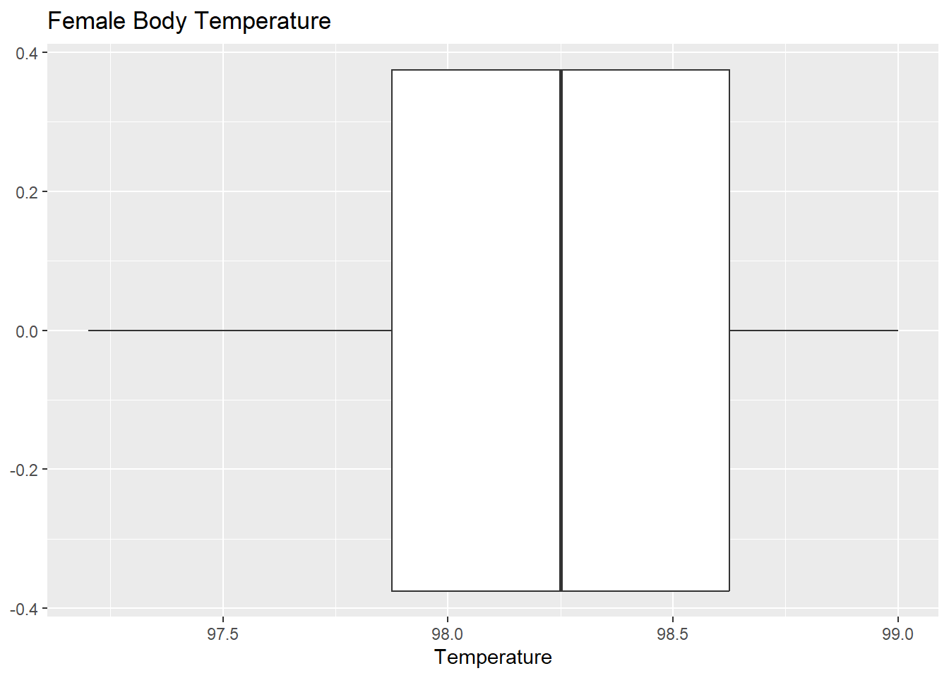

Code

df_prob1 %>%
  t.test(alternative = c("two.sided"),
         mu = 98.6,
         paired = FALSE,
         var.equal = FALSE)


    One Sample t-test

data:  .
t = -2.8824, df = 15, p-value = 0.01139
alternative hypothesis: true mean is not equal to 98.6
95 percent confidence interval:
 97.92596 98.49904
sample estimates:
mean of x 
  98.2125

Code

#Computing the Test Statistic###########################################
df_prob2 %>%
  ggplot() + 
  geom_density(
    aes(x = Before, fill = "Before"),
    alpha = 0.5) +
  geom_density(
    aes(x = After, fill = "After"),
    alpha = 0.5)+
  ggtitle("Delay Time Before vs After Alteration")+
  xlab("Delay Time")

Warning: Removed 1 rows containing non-finite values (`stat_density()`).
Removed 1 rows containing non-finite values (`stat_density()`).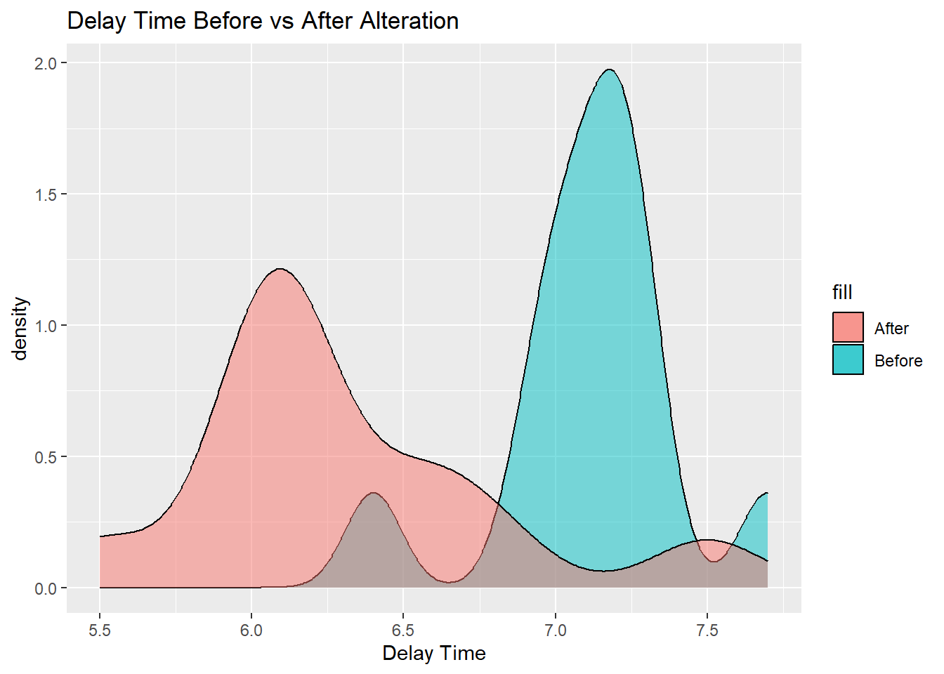

Code

df_prob2 %$%
  z.test(
    Before,
    After,
    alternative = c("less"),
    mu = 1,
    sigma.x = 0.3, sigma.y = 0.3,
    conf.level = 0.90)


    Two-sample z-Test

data:  Before and After
z = -1.4289, p-value = 0.07652
alternative hypothesis: true difference in means is less than 1
90 percent confidence interval:
        NA 0.9819574
sample estimates:
mean of x mean of y 
 7.116667  6.291667

Code

#Computing the Test Statistic######################################################
df_prob3 %>%
  ggplot()+
  geom_boxplot(aes(BrandOne), fill = "lightslategray")+
  geom_boxplot(aes(BrandTwo), fill = "mediumaquamarine")+
  ggtitle("Distance by Golf Ball Brand")+
  xlab("Brand 1 vs Brand 2")

Warning: Removed 1 rows containing non-finite values (`stat_boxplot()`).

Warning: Removed 1 rows containing non-finite values (`stat_boxplot()`).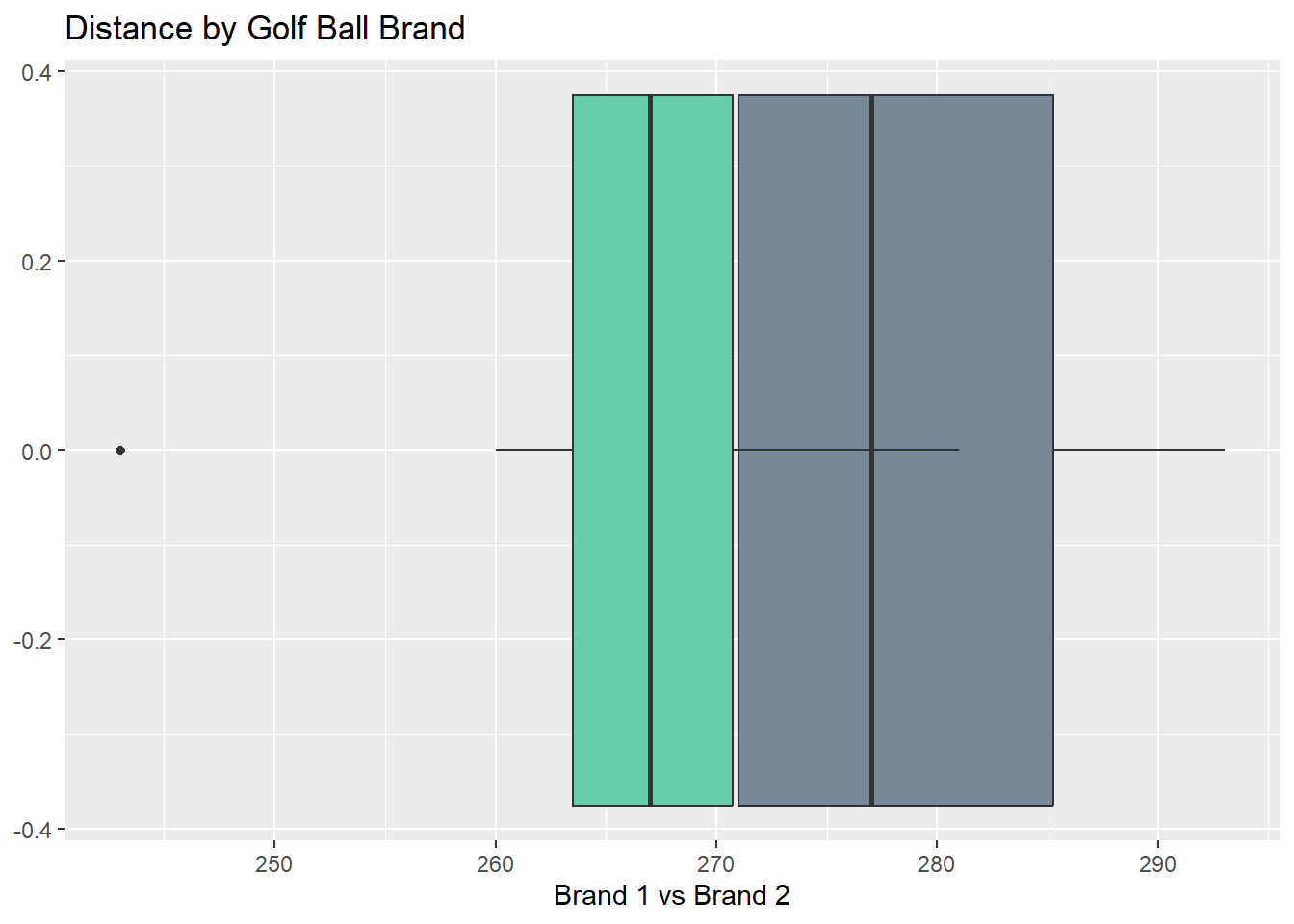

Code

df_prob3 %$%
  t.test(
    BrandOne,
    BrandTwo,
    alternative = c("two.sided"),
    var.equal=TRUE,
    mu = 0)


    Two Sample t-test

data:  BrandOne and BrandTwo
t = 2.6151, df = 18, p-value = 0.01753
alternative hypothesis: true difference in means is not equal to 0
95 percent confidence interval:
  2.260984 20.739016
sample estimates:
mean of x mean of y 
    277.5     266.0

Code

#Computing the Test Statistic###########################################
df_prob4 %>%
  ggplot()+
  geom_density(
    aes(x = SolutionOne, fill = "SolutionOne"),
    alpha = 0.5)+
  geom_density(
    aes(x = SolutionTwo, fill = "SolutionTwo"),
    alpha = 0.5)+
  ggtitle("Etch Rates of Solutions")+
  xlab("Solution 1 vs Solution 2")

Warning: Removed 1 rows containing non-finite values (`stat_density()`).

Warning: Removed 1 rows containing non-finite values (`stat_density()`).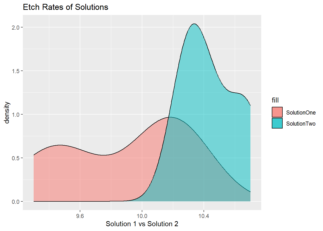

Code

df_prob4 %$%
  t.test(
    SolutionOne,
    SolutionTwo,
    alternative = c("two.sided"),
    var.equal=TRUE,
    mu = 0)


    Two Sample t-test

data:  SolutionOne and SolutionTwo
t = -4.0101, df = 18, p-value = 0.0008211
alternative hypothesis: true difference in means is not equal to 0
95 percent confidence interval:
 -0.838149 -0.261851
sample estimates:
mean of x mean of y 
     9.89     10.44

Code

#Computing the Test Statistic###############################################
df_prob5 %>%
  ggplot()+
  geom_density(
    aes(x = FacilityOne, fill = "FacilityOne"),
    alpha = 0.5)+
  geom_density(
    aes(x = FacilityTwo, fill = "FacilityTwo"),
    alpha = 0.5)+
  ggtitle("Water Hardness by Facility")+
  xlab("Facility 1 vs Facility 2")

Warning: Removed 2 rows containing non-finite values (`stat_density()`).
Removed 1 rows containing non-finite values (`stat_density()`).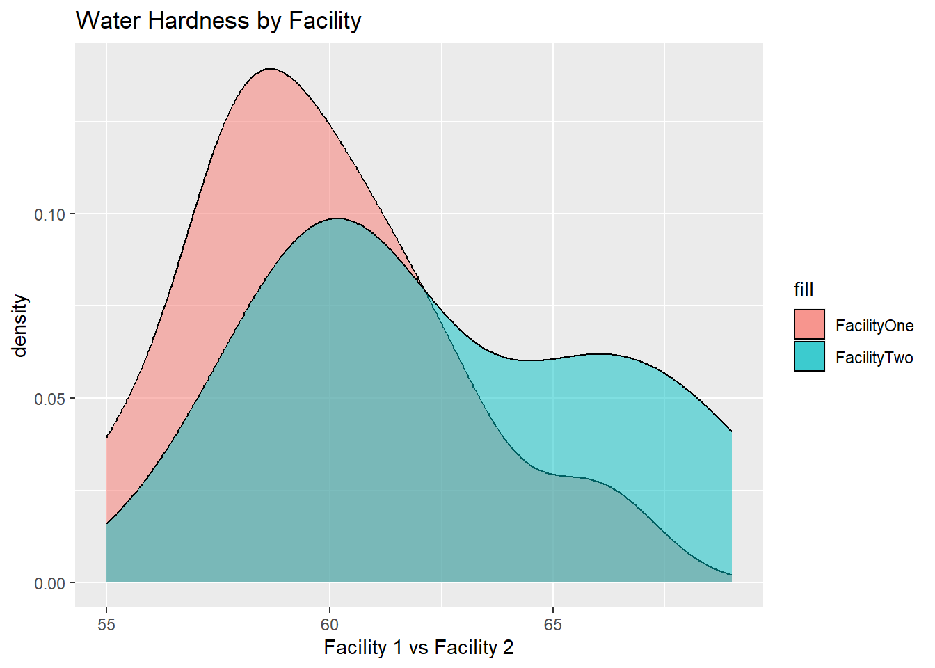

Code

df_prob5 %$%
  t.test(
    FacilityOne,
    FacilityTwo,
    alternative = c("two.sided"),
    var.equal=TRUE,
    mu = 0)


    Two Sample t-test

data:  FacilityOne and FacilityTwo
t = -2.0275, df = 23, p-value = 0.05436
alternative hypothesis: true difference in means is not equal to 0
95 percent confidence interval:
 -5.6335904  0.0566673
sample estimates:
mean of x mean of y 
 59.75000  62.53846

Code

df_prob5 %$%
  t.test(
    FacilityOne,
    FacilityTwo,
    alternative = c("two.sided"),
    var.equal=FALSE,
    mu = 0)


    Welch Two Sample t-test

data:  FacilityOne and FacilityTwo
t = -2.0488, df = 22.358, p-value = 0.0524
alternative hypothesis: true difference in means is not equal to 0
95 percent confidence interval:
 -5.60847479  0.03155171
sample estimates:
mean of x mean of y 
 59.75000  62.53846

See the figure below for context regarding the conclusions drawn for each individual problem statement. The null and alternate hypotheses mentioned in the document refer to the real-world, practical scenarios in the problem statements associated with the data set.